Closeness Centrality
We all have an intuitive understanding when we say a home, an office, or a store is "centrally located." Something that is centrally located is roughly equidistant from several destinations.
Closeness Centrality provides a precise measure of how "centrally located" all the vertices are.
The steps below show the steps for one vertex v:
| Step | Mathematical Formula |
|---|---|
1. Compute the average distance from vertex v to every other vertex: |
\(d_{avg}(v) = \sum_{u \ne v} dist(v,u)/(n-1)\) |
2. Invert the average distance, so we have average closeness of v: |
\(CC(v) = 1/d_{avg}(v)\) |
This is repeated across all vertices in the graph.
Notes
This algorithm query employs a subquery called cc_subquery.
Both queries are needed to run the algorithm.
The re_type (reverse edge type) parameter is always required.
For undirected edges, use the same value for both e_type and re_type.
References
TigerGraph’s closeness centrality algorithm uses multi-source breadth-first search (MS-BFS) to traverse the graph and calculate the sum of a vertex’s distance to every other vertex in the graph, which vastly improves the performance of the algorithm.
The algorithm’s implementation of MS-BFS is based on the paper The More the Merrier: Efficient Multi-source Graph Traversal by Then et al.
Specifications
tg_closeness_cent (SET<STRING> v_type, SET<STRING> e_type, INT max_hops=10,
  INT top_k=100, BOOL wf = TRUE, BOOL print_accum = True, STRING result_attr = "",
  STRING file_path = "", BOOL display_edges = FALSE)
Parameters
| Parameter | Description | Default |
|---|---|---|
|
Vertex types to use |
(empty set of strings) |
|
Edge types to use |
(empty set of strings) |
|
Reverse edge types to use |
(empty set of strings) |
|
If >=0, look only this far from each vertex |
10 |
|
Output only this many scores (scores are always sorted highest to lowest) |
100 |
|
Whether to use Wasserman-Faust normalization for multi-component graphs |
True |
|
If True, output JSON to standard output |
True |
|
If not empty, store centrality values in |
(empty string) |
|
If not empty, write output to this file in CSV format. |
(empty string) |
|
If true, include the graph’s edges in the JSON output so that the full graph can be displayed. |
False |
Example
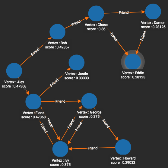
Closeness centrality can be measured for either directed edges (from v to others) or for undirected edges. Directed graphs may seem less intuitive, however, because if the distance from Alex to Bob is 1, it does not mean the distance from Bob to Alex is also 1.
For our example, we wanted to use the topology of a friendship graph, but to have undirected edges. We emulated an undirected graph by using both Friend and Also_Friend (reverse-direction) edges.
# Use _ for default values
RUN QUERY tg_closeness_cent(["Person"], ["Friend", "Also_Friend"], _, _,
_, _, _, _, _)