Betweenness Centrality
The Betweenness Centrality of a vertex is defined as the number of shortest paths that pass through this vertex, divided by the total number of shortest paths. That is
where \(PD\) is the pair dependency, \(SP_{st}\)is the total number of shortest paths from node s to node t and \(SP_{st}(v)\)is the number of those paths that pass through v.
The TigerGraph implementation is based on A Faster Algorithm for Betweenness Centrality by Ulrik Brandes, Journal of Mathematical Sociology 25(2):163-177, (2001).
For every vertex s in the graph, the pair dependency starting from vertex s to all other vertices t via all other vertices v is computed first:
Then betweenness centrality is computed as
According to Brandes, the accumulated pair dependency can be calculated as
where \(P_s(w)\), the set of predecessors of vertex w on shortest paths from s, is defined as
For every vertex, the algorithm works in two phases. The first phase calculates the number of shortest paths passing through each vertex. Then starting from the vertex on the most outside layer in a non-incremental order with pair dependency initial value of 0, traverse back to the starting vertex.
Notes
This query algorithm employs a subquery called bc_subquery. Both queries are needed to run the algorithm.
Specifications
CREATE QUERY tg_betweenness_cent(SET<STRING> v_type, SET<STRING> e_type,
STRING re_type,INT max_hops=10, INT top_k=100, BOOL print_accum = True,
STRING result_attr = "", STRING file_path = "", BOOL display_edges = FALSE)
Parameters
| Parameter | Description | Default Value |
|---|---|---|
|
The vertex types to use |
(empty set of strings) |
|
The edge types to use |
(empty set of strings) |
|
The reverse edge types to use |
(empty set of strings) |
|
If >=0, look only this far from each vertex |
10 |
|
The number of scores to output, sorted in descending order |
100 |
|
If true, print output in JSON format to the standard output. |
True |
|
If not empty, store centrality values in |
(empty string) |
|
If not empty, write output to this file. |
(empty string) |
|
If true, include the graph’s edges in the JSON output, so that the full graph can be displayed. |
True |
Output
Computes a Betweenness Centrality value (FLOAT type) for each vertex.
The result size is equal to \(V\), the number of vertices.
Time complexity
This algorithm has a time complexity of \(O(E*V)\) where \(E\) is the number of edges and \(V\) is the number of vertices.
Considering the high time cost of running this algorithm on a big graph, users can set a maximum number of iterations. Parallel processing reduces the time needed for computation.
Example
In this example, Claire is in the very center of the graph and has the highest betweenness centrality. Six shortest paths pass through Sam (i.e. paths from Victor to all other 6 people except for Sam and Victor), so the score of Sam is 6. David also has a score of 6, since Brian has 6 paths to other people that pass through David.
# Use _ for default values
RUN QUERY tg_betweenness_cent(["Person"], ["Friend"], _, _, _, _, _, _)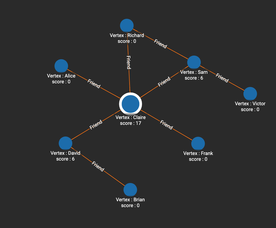
[
{
"@@BC": {
"Alice": 0,
"Frank": 0,
"Claire": 17,
"Sam": 6,
"Brian": 0,
"David": 6,
"Richard": 0,
"Victor": 0
}
}
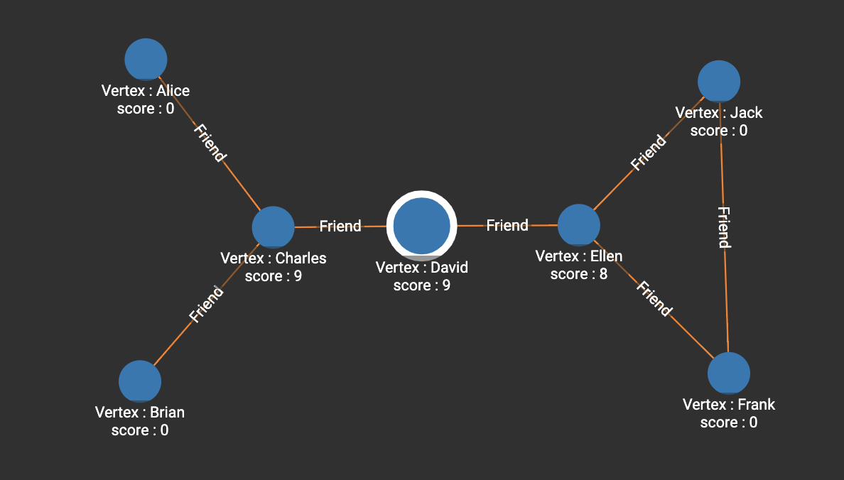
]In the following example, both Charles and David have 9 shortest paths passing through them. Ellen is in a similar position as Charles, but her centrality is weakened due to the path between Frank and Jack.
[
  {
    "@@BC": {
      "Alice": 0,
      "Frank": 0,
      "Charles": 9,
      "Ellen": 8,
      "Brian": 0,
      "David": 9,
      "Jack": 0
    }
  }
]