Jaccard Similarity of Neighborhoods (Single Source)
The Jaccard index measures the relative overlap between two sets.
To compare two vertices by Jaccard similarity, first select a set of attribute values for each vertex.
For example, a set of values for a Person vertex could be the list of cities the person has lived in. The Jaccard index is computed for the two value sets.
The Jaccard index of two sets A and B is defined as follows:
The value ranges from 0 to 1. If A and B are identical, then \(Jaccard(A, B) = 1\). If both A and B are empty, we define the value to be 0.
Specifications
tg_jaccard_nbor_ss (VERTEX source, STRING e_type, STRING rev_e_type,  INT top_k = 100,
  BOOL print_accum = TRUE, STRING similarity_edge_type = "",STRING file_path = "")
Parameters
| Parameter | Description | Default value |
|---|---|---|
|
Vertex type used to calculate similarity score |
(empty set of strings) |
|
Edge type to traverse |
(empty set of strings) |
|
Reverse edge type to traverse |
(empty set of strings) |
|
The number of vertex pairs with the highest similarity scores to return. Limits number of returned items. |
100 |
|
Whether to output the final results to the console in JSON format |
True |
|
If provided, the similarity score will be saved to this edge |
(empty string) |
|
If provided, the algorithm will save the output in CSV format to this file |
(empty string) |
Output
The top k vertices in the graph that have the highest similarity scores, along with their scores.
Vertices with a similarity score of 0 to the target vertex are not included.
The result is available in three forms:
-
streamed out in JSON format
-
written to a file in tabular format, or
-
stored as a vertex attribute value.
Example
This example uses a Movie Rating graph consisting of Person and Movie vertices. There are Likes edges that are weighted according to how much the person liked the movie. Each person in the dataset liked at least one movie, but not all movies were liked by all people.
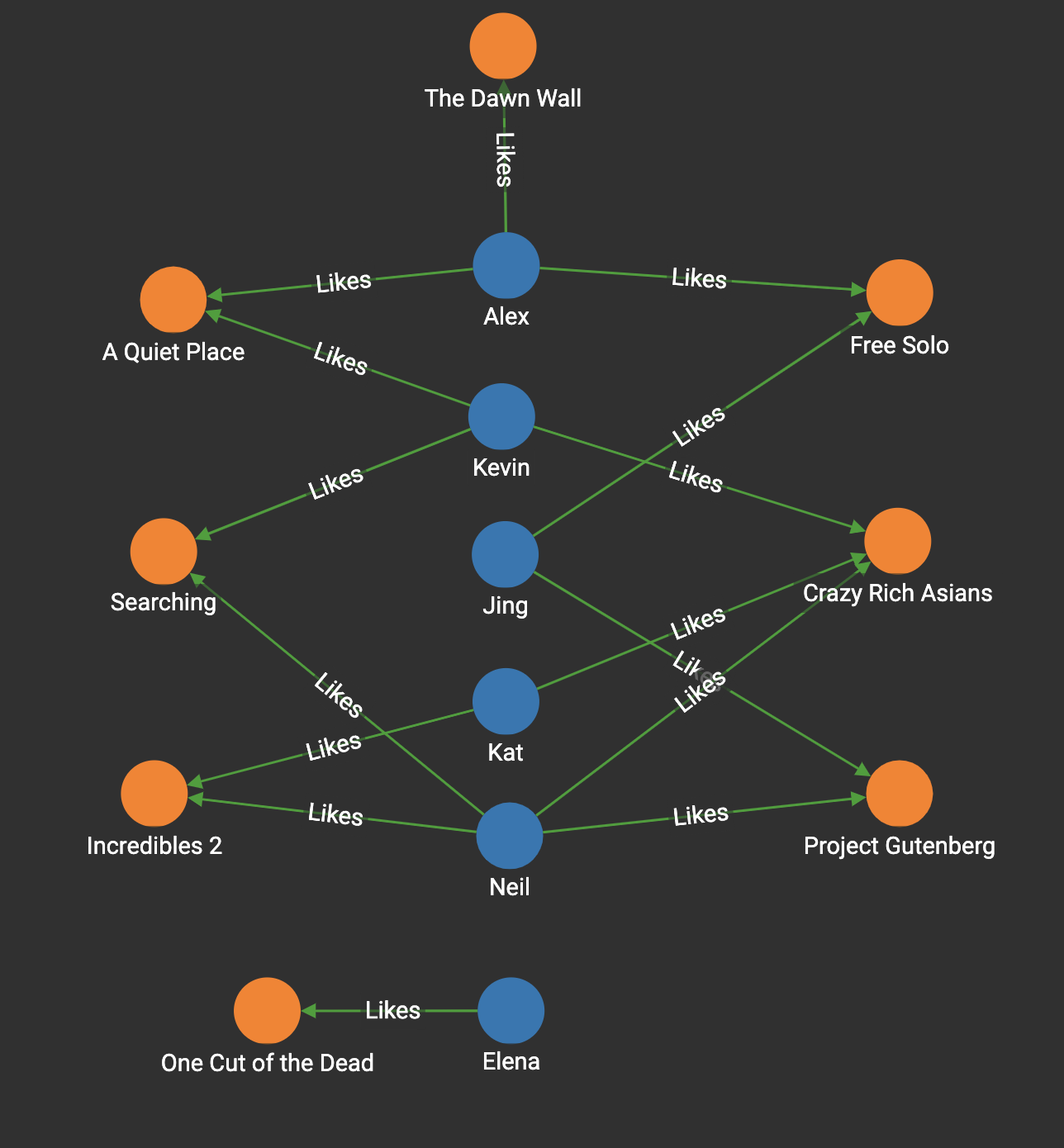
Here we run tg_jaccard_nbor_ss("Neil", "Likes", "Reverse_Likes", 5):
[
  {
    "Others": [
      {
        "attributes": {
          "Others.@sum_similarity": 0.5
        },
        "v_id": "Kat",
        "v_type": "Person"
      },
      {
        "attributes": {
          "Others.@sum_similarity": 0.4
        },
        "v_id": "Kevin",
        "v_type": "Person"
      },
      {
        "attributes": {
          "Others.@sum_similarity": 0.2
        },
        "v_id": "Jing",
        "v_type": "Person"
      }
    ]
  }
]
When comparing similarity to Neil, Kat is ranked higher than Kevin. This makes intuitive sense, because Kat likes two movies, both of which were also liked by Neil. Kevin also likes two movies that Neil likes. However, Kevin also likes a third movie that Neil doesn’t like, and is therefore less similar than Kat was.
Although we set top_k to 5, only three vertices were returned because neither Alex nor Elena likes any movies that Kevin likes.
If the source vertex (Person) doesn’t have any common neighbors (Movies) with any other vertex (Person), such as Elena in our example, the result is an empty list:
Here we run tg_jaccard_nbor_ss("Elena", "Likes", "Reverse_Likes", 5):
[
  {
    "Others": []
  }
]