Single-source Shortest Path (Weighted)
Updated 15 Oct 2024 to document the overlooked epsilon parameter.
|
Finding shortest paths in a graph with weighted edges is algorithmically harder than in an unweighted graph because even after you find one path to a vertex T, you cannot be certain that it is a shortest path.
If edge weights are always positive, then you must keep trying until you have considered every in-edge to T. If edge weights can be negative, then it’s even harder. You must consider all possible paths.
A classic application for a weighted shortest path algorithm is finding the shortest travel route to get from an origin location to a destination location. In this case, the edge weights would be the distances between vertices. In general, any application where you are looking for the cheapest route is a possible fit.
Notes
If you have edges with positive weights, use shortest_path_pos_wt, which is based on the delta-stepping approach, to take advantage of TigerGraph’s parallel processing.
Each round, the algorithm tries to find a shorter path to each destination.
epsilon (aka delta) is the minimum path reduction the algorithm must find in a round in order to justify searching for another round.
The well-known Dijsktra’s algorithm is not well-suited for parallel computation.
If you have edges with both positive and negative weights, use shortest_path_any_wt, which implements the Bellman-Ford algorithm.
If there is more than one path with the same total weight, the algorithm returns one of them.
Specifications
The shortest path algorithm can be optimized if we know all the weights are non-negative. If there can be negative weights, then sometimes a longer path will have a lower cumulative weight. Therefore, we have two versions of this algorithm
tg_shortest_ss_pos_wt (VERTEX source,  SET<STRING> v_type_set,  SET<STRING> e_type_set,
 STRING weight_attribute, STRING weight_type, FLOAT epsilon = 0.001,
INT print_limit = -1, BOOL print_results = TRUE,
 STRING result_attribute = "", STRING file_path = "", BOOL display_edges = FALSE)
tg_shortest_ss_any_wt (VERTEX source, SET<STRING> v_type_set, SET<STRING> e_type_set,
STRING weight_attribute, STRING weight_type, INT print_limit = -1, BOOL print_results = TRUE,
STRING result_attribute = "", STRING file_path = "", BOOL display_edges = FALSE)Parameters
| Parameter | Description | Default |
|---|---|---|
|
The source vertex to start from. Provide the vertex ID and type as a tuple: |
(empty string) |
|
Names of vertex types to use |
(empty string) |
|
Names of edge types to use |
N/A |
|
Name of the edge weight attribute |
(empty string) |
|
The data type of the edge weight attribute.
Can be |
(empty string) |
|
Minimum delta weight. |
0.001 |
|
If >=0, max number of vertices to output to JSON |
-1 |
|
Whether to print results in JSON format to standard output |
True |
|
If not empty, store distance values in INT to this vertex attribute |
(empty string) |
|
If not empty, write output to this file. |
(empty string) |
|
If true, include the graph’s edges in the JSON output, so that the full graph can be displayed in the query view window on GraphStudio. |
False |
Example
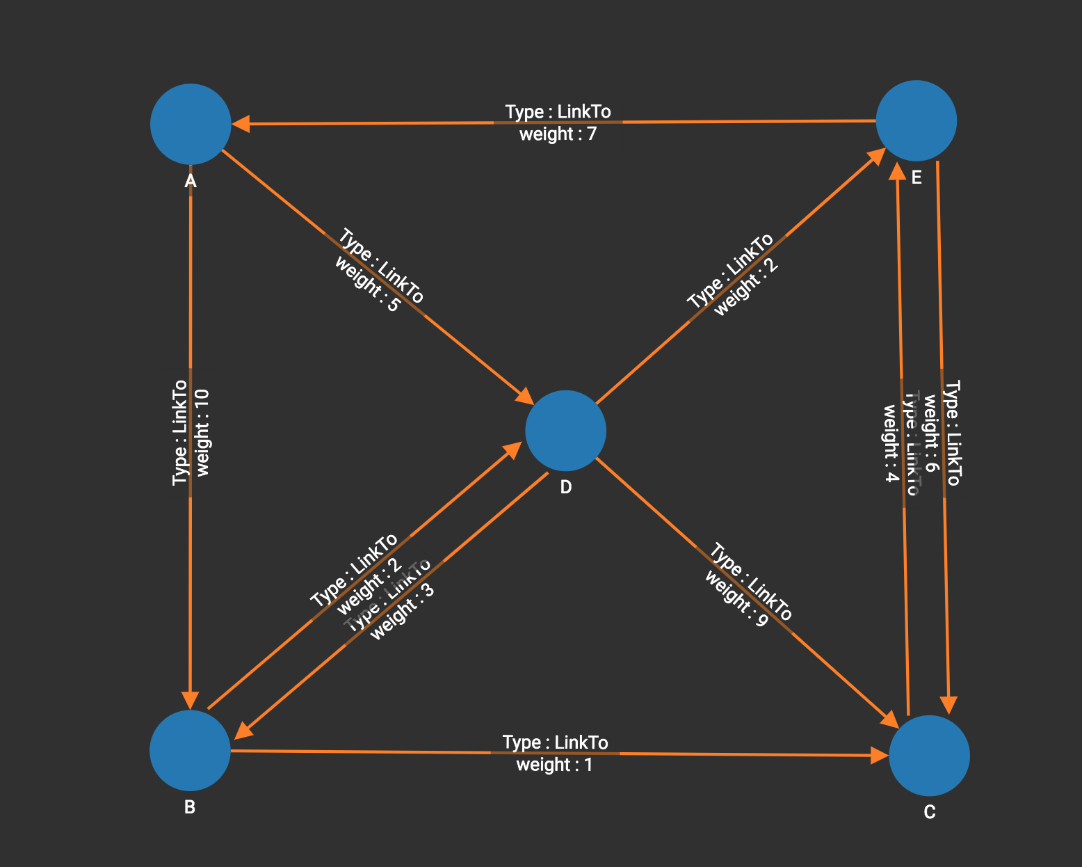
The graph below has only positive edge weights. Using vertex A as the source vertex, the algorithm discovers that the shortest weighted path from A to B is A-D-B, with distance 8. The shortest weighted path from A to C is A-D-B-C with distance 9.

[
  {
    "ResultSet": [
      {
        "v_id": "B",
        "v_type": "Node",
        "attributes": {
          "ResultSet.@dis": 8,
          "ResultSet.@path": [
            "D",
            "B"
          ]
        }
      },
      {
        "v_id": "A",
        "v_type": "Node",
        "attributes": {
          "ResultSet.@dis": 0,
          "ResultSet.@path": []
        }
      },
      {
        "v_id": "C",
        "v_type": "Node",
        "attributes": {
          "ResultSet.@dis": 9,
          "ResultSet.@path": [
            "D",
            "B",
            "C"
          ]
        }
      },
      {
        "v_id": "E",
        "v_type": "Node",
        "attributes": {
          "ResultSet.@dis": 7,
          "ResultSet.@path": [
            "D",
            "E"
          ]
        }
      },
      {
        "v_id": "D",
        "v_type": "Node",
        "attributes": {
          "ResultSet.@dis": 5,
          "ResultSet.@path": [
            "D"
          ]
        }
      }
    ]
  }
]
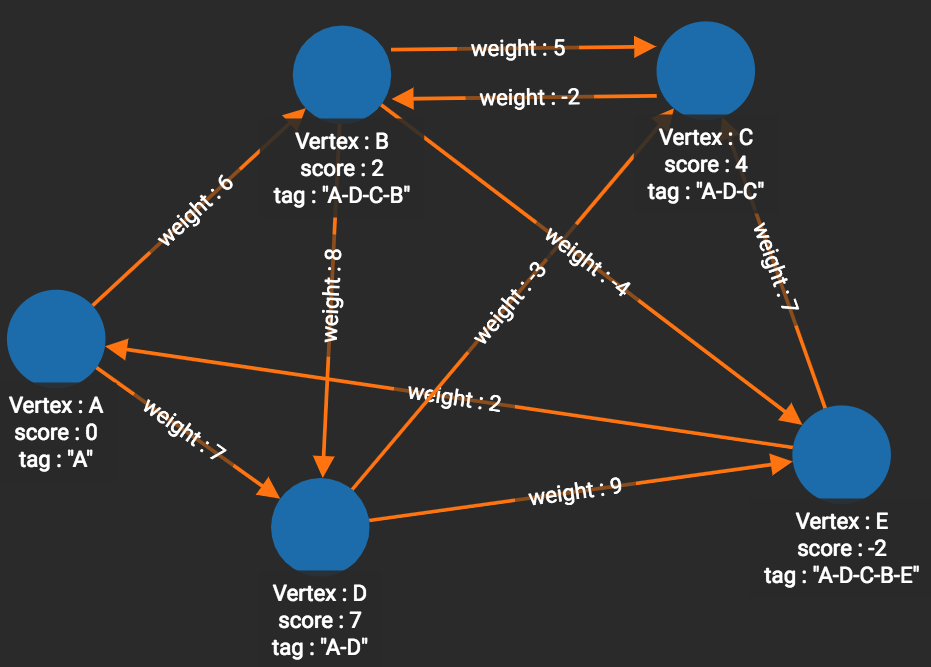
The graph below has both positive and negative edge weights. Using vertex A as the source vertex, the algorithm discovers that the shortest weighted path from A to E is A-D-C-B-E, with a cumulative score of 7 - 3 - 2 - 4 = -2.
